Building a Technical Trading Data & Analytics Pipeline

Background

As a person with a strong background in analytics and a love of programming, I’ve always wanted to have a go at technical investing, using my own pipeline. I’ve finally taken the project on in earnest, and I’m going to chronicle the twists and turns it takes on the blog—this is Part 1.

So, what do I mean by ‘pipeline’ in this context? Essentially, I mean ingesting market data, algorithmically curating buy candidates, tracking existing positions for sell signals, and all the nitty gritty in-betweens that entails. I envision four high-level components:

1. Data ingestion and transformation,

2. Application of a model to identify and rank buy candidates,

3. Daily, automated report creation to help me make decisions on buy candidates, and

4. Daily/intraday reporting/monitoring for existing positions.

I’ve started on numbers 1 and 3, so I will cover some of that here.

Data Ingestion

I’m going to focus exclusively on stocks to start, and I’ll be getting my data from Polygon.io—they have a variety of data offerings across various personal and business tiers (including a free option). I’ll be using the Stocks Starter plan, which provides a decent amount of historical data aggregated in flat files by day or minute via Amazon S3 as well as near-real-time data via API.

My core data object that will serve as input to the curation model will be a Python (Polars) DataFrame of daily aggregates for all U.S. stocks (~10K) over a flexible window of time through the prior trading day. I’ll build the DataFrame from flat files using the Python Boto3 SDK for S3 and two custom functions.

Function 1: List Files

This function returns a list of file names satisfying parameterized criteria (day vs. minute, last day, window size, etc.).

def list_hist_files(
        kind='day_aggs',
        last_day='2025-03-28',
        window=30,
        prefix='us_stocks_sip',
        bucket_name='flatfiles',
        bookend=False,
    ):

    session=boto3.Session(
        aws_access_key_id=aws_access_key_id,
        aws_secret_access_key=aws_secret_access_key,
    )

    s3=session.client(
        's3',
        endpoint_url='https://files.polygon.io',
        config=Config(signature_version='s3v4'),
    )

    paginator=s3.get_paginator('list_objects_v2')

    dates=[]
    end_date=datetime.strptime(last_day,'%Y-%m-%d')
    for delta in range(window+1):
        temp_past_date=end_date-timedelta(days=delta)
        dates.append(datetime.strftime(temp_past_date,'%Y-%m-%d'))

    files=[]
    for page in paginator.paginate(Bucket=bucket_name, Prefix=prefix):
        for obj in page['Contents']:
            if obj['Key'].find(kind)>=0 and re.sub('.*(\\d{4}-\\d{2}-\\d{2}).*','\\1',obj['Key']) in dates: 
                files.append(obj['Key'])

    if bookend and len(files)>2:
        files=[files[0],files[-1]]

    return files

Function 2: Ingest Files

The second function reads a single, dated file for the full market or for an optional subset of tickers into memory and returns a Polars DataFrame. This function has a simple positional parameterization, as it’s intended to be called via the itertools.starmap() functional.

def get_hist_data(file,tickers):

    date=re.sub('.*(\\d{4}-\\d{2}-\\d{2}).*','\\1',file)

    session=boto3.Session(
        aws_access_key_id=aws_access_key_id,
        aws_secret_access_key=aws_secret_access_key,
    )

    s3=session.client(
        's3',
        endpoint_url='https://files.polygon.io',
        config=Config(signature_version='s3v4'),
    )

    response=s3.get_object(Bucket='flatfiles',Key=file)
    compressed_data=response["Body"].read()

    with gzip.GzipFile(fileobj=io.BytesIO(compressed_data),mode="rb") as f:
        if tickers: df=pl.scan_csv(f).filter(pl.col('ticker').is_in(tickers)).collect()
        else: df=pl.read_csv(f)

    return df.insert_column(1,pl.lit(date).alias("date"))

Data Transformation

Next, I pull in the data and create some metrics, including candlesticks, short and long simple moving averages, moving average convergence/divergence (MACD) indicator and signal (its moving average), and the relative strength index (RSI). Note that I convert to a Pandas DataFrame here to make the data readable in a subsequent R block—that’s just a byproduct of this post being written in Quarto. This portion of the pipeline will be scripted when implemented.

import polars as pl
import itertools as it
import boto3
from botocore.config import Config
import tempfile
import gzip
import io
import re
from datetime import datetime, timedelta
from polygon import RESTClient
import polars.selectors as cs
from dataclasses import asdict

with open("/Users/lance/Desktop/TechInvest/scripts/sandbox/01_GetHistAggs.py") as script:
    exec(script.read())

with open("/Users/lance/Desktop/TechInvest/keys.py") as script:
    exec(script.read())

iterator=it.product(
    list_hist_files(kind="day_aggs",last_day=r.params["ref_date"],window=r.params["window"],bookend=False),
    [[r.params["ticker"]]],
)

df=it.starmap(get_hist_data,iterator)

df=(
    pl.concat(list(df))
    .lazy()
    .sort("ticker","window_start")
    .with_columns(
        pl.col("close").rolling_mean(window_size=r.params["sma_l"]).over("ticker").alias("sma_l"),
        pl.col("close").rolling_mean(window_size=r.params["sma_s"]).over("ticker").alias("sma_s"),
        (pl.col("close").ewm_mean(span=12,min_samples=12)-
            pl.col("close").ewm_mean(span=26,min_samples=26)
        ).over("ticker").alias("MACD"),
        (pl.col("close")*2-pl.col("close").rolling_sum(window_size=2)).over("ticker").alias("rsi_diff"),
        pl.when(pl.col("close")>pl.col("open")).then(1)
        .otherwise(-1)
        .alias("candle_color"),
        pl.max_horizontal("open","close").alias("candle_high"),
        pl.min_horizontal("open","close").alias("candle_low"),
        pl.mean_horizontal("open","close").alias("candle_mid"),
    )
    .with_columns(
        pl.col("MACD").ewm_mean(span=9,min_samples=9).over("ticker").alias("signal"),
        pl.when(pl.col("rsi_diff")>0).then("rsi_diff")
        .otherwise(0)
        .alias("U"),
        pl.when(pl.col("rsi_diff")<0).then(-pl.col("rsi_diff"))
        .otherwise(0)
        .alias("D"),
    )
    .with_columns(
        (pl.col("MACD")-pl.col("signal")).alias("histogram"),
        ((pl.col("U").ewm_mean(min_samples=14,alpha=1/14))/(pl.col("D").ewm_mean(min_samples=14,alpha=1/14))).alias("RS"),
    )
    .with_columns((100-100/(1+pl.col("RS"))).alias("RSI"))
    .filter(pl.col("signal").is_not_null())
    .collect()
    .to_pandas()
)

A Graphics Template for Buy Candidate Analysis and Position Monitoring

I could probably develop these graphics in Python, but I’ve just got way too much ggplot experience at this point and would rather do this part in R. The idea is to present a consistent set of metrics I can use to make buy/sell decisions. I think these will be embedded in ticker-specific html reports along with other relevant information as of yet undetermined. Here’s the code with some example output for NVIDIA stock over a 10-week window ending on April 1, 2025.

library(tidyverse)
library(reticulate)
library(patchwork)
library(ggthemes)

bg<-"#7AD151FF"
r<-"#31688EFF"

hotline<-"#FDE725FF"
coldline<-"#1F988BFF"

theme<-theme_set(theme_solarized(light=FALSE))+
    theme_update(
        axis.text.x=element_blank(),axis.ticks.x=element_blank(),
        axis.text.y=element_text(color="#bbbbbb")
    )

g2<-ggplot(py$df,aes(x=as_date(date)))+
    geom_hline(yintercept=0,linewidth=.5,color="#111111")+
    geom_col(aes(y=histogram,fill=MACD>signal),color="#111111")+
    scale_x_date(
        limits=c(min(as_date(py$df$date))-1,max(as_date(py$df$date))+1),
        date_breaks="1 week",
        date_minor_breaks="1 day",
        expand=expansion(add=0),
    )+
    scale_y_continuous()+
    scale_fill_manual(values=c(r,bg))+
    labs(y=NULL,x=NULL)+
    guides(color="none",fill="none")

u<-layer_scales(g2)$x$limits[[2]] %>% as_date()
l<-layer_scales(g2)$x$limits[[1]] %>% as_date()

g1<-ggplot(py$df,aes(x=as_date(date)))+
    geom_hline(yintercept=0,linetype=2,linewidth=.5,color="#bbbbbb")+
    geom_line(aes(y=signal),color=coldline,linewidth=1.1)+
    geom_line(aes(y=MACD),color=hotline,linewidth=1.1)+
    scale_x_date(
        limits=c(l,u),
        date_breaks="1 week",
        date_minor_breaks="1 day",
        expand=expansion(add=0),
    )+
    scale_y_continuous()+
    labs(y=NULL,x=NULL)+
    guides(color="none",fill="none")

g3<-ggplot(py$df,aes(x=as_date(date)))+
    theme_update(
        axis.text.x=element_text(angle=45,hjust=1,vjust=1,color="#bbbbbb"),
        axis.ticks.x=element_line(),
    )+
    geom_line(aes(y=RSI),linewidth=1.1,color=hotline)+
    annotate(
        geom="rect",
        fill=coldline,
        xmin=l,
        xmax=u,
        ymin=30,
        ymax=70,
        alpha=0.5,
    )+
    scale_x_date(
        limits=c(l,u),
        date_breaks="1 week",
        date_minor_breaks="1 day",
        expand=expansion(add=0),
    )+
    scale_y_continuous(limits=c(0,100),breaks=c(0,30,70,100))+
    labs(y=NULL,x=NULL)+
    guides(color="none",fill="none")+
    theme_update(
        axis.text.x=element_blank(),
        axis.ticks.x=element_blank(),
    )

p<-ggplot(py$df,aes(x=as_date(date)))+
    geom_line(aes(y=sma_l),color=coldline,linewidth=1.1)+
    geom_line(aes(y=sma_s),color=hotline,linewidth=1.1)+
    geom_linerange(aes(ymax=high,ymin=low,color=factor(candle_color)),linewidth=1.1)+
    geom_tile(
        aes(
            y=candle_mid,
            height=candle_high-candle_low,
            fill=factor(candle_color),
        ),
        width=.8,
        linewidth=.4,
        color="#111111",
    )+
    scale_x_date(
        limits=c(l,u),
        date_breaks="1 week",
        date_minor_breaks="1 day",
        expand=expansion(add=0),
    )+
    scale_fill_manual(values=c(r,bg))+
    scale_color_manual(values=c(r,bg))+
    scale_y_continuous(labels=scales::dollar)+
    labs(y=NULL,x=NULL)+
    ggtitle(str_glue("Ticker: {params$ticker}"))+
    guides(color="none",fill="none")

p / g1 / g2 / g3 + plot_layout(nrow=4,heights=c(3,1,1,1))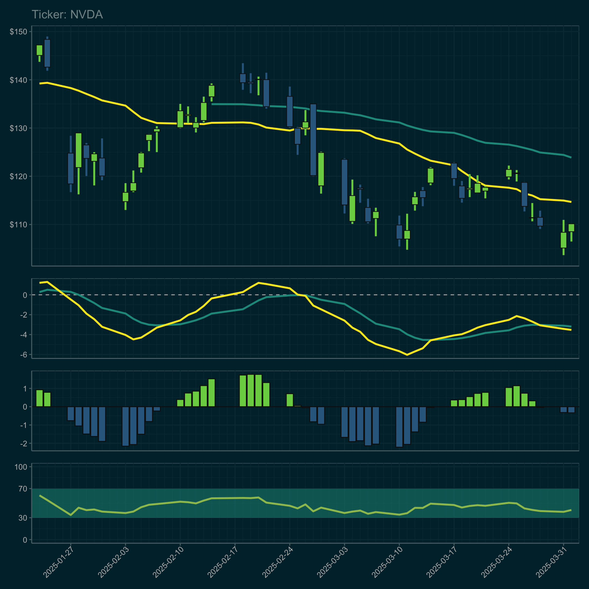

Much more to come, but that’s it for now!